 |
|
Methods for Establishing Receiving Water Quality Impacts of Urban and Suburban Development
This summary was developed by USEPA Region 5 - Chicago.
I. INTRODUCTION
This chapter provides an overview of practical methods for estimating short-term and long-term surface water quality impacts related to urban and suburban development sites. These methods may be used by the urban planner or developer to estimate the impacts on receiving waters from development which may result based on various planning conditions and assumptions. Using the approaches presented here, mitigation of water quality impacts may be tested based upon incorporation of various types of management practices.
II. IMPACTS OF URBAN AND SUBURBAN DEVELOPMENT
There are two principal types of water quality impacts typically associated with urban and suburban development. The first includes the impacts related to the construction phase of development as soils which are destabilized due to clearing grading and excavation are subject to increased erosion by wind and water. Eroded soils associated with construction activity can be carried offsite and deposited in receiving waters such as lakes, rivers and wetlands. Adverse impacts related to these sediments include increased turbidity and habitat modification, including smothering of spawning beds. While the construction phase itself may be relatively short-lived, the impacts to receiving waters from poorly managed construction activities may be extremely severe and long-lasting, particularly to sensitive areas such as wetlands and inland lakes.
Once the construction phase is over, other receiving water quality impacts may become more pronounced due to potentially dramatic changes to the area's hydrology (reduced baseflow and exaggerated peak flow volumes), and the change in land use compared to predevelopment conditions. The increase in impervious areas causes a resultant increase in runoff rates and volumes. This can result in increased streambank erosion and associated water quality problems.
The increased runoff also accelerates the transport of land-borne pollutants into receiving waters. Typical pollutants which may be found in urban storm water at significant levels include heavy metals, oil and grease, pesticides, fertilizers and other nutrients, and toxic organic contaminants. Runoff from roadways and parking lots may cause significant elevations in receiving water temperatures during summer months. Winter road deicing activities can contribute high levels of chlorides or sediment.
In order to properly manage and maintain urban water resources, the impacts associated with new development must be carefully evaluated. Post-development impacts may be evaluated in terms of short-term (acute) impacts, and long-term (chronic) impacts. Short term impacts include the changes to a receiving water's chemistry, hydrology, temperature, etc, caused by individual runoff events, and are typically on a timescale of hours to days. Long-term impacts are those which are manifested in the weeks-to-years timescale, and include changes to the dry and wet weather hydrology, streambank morphology, and water chemistry of the receiving water. Long-term chemical impacts are most critical for receiving waters with longer residence times such as lakes and wetlands, and for slower moving stream segments.
In terms of the changes to a receiving water's chemistry due to urban runoff, pollutant concentrations are best used to evaluate short-term effects, while pollutant loadings are appropriate for assessing long-term impacts. Land use planners and developers need to understand these impacts and carefully plan in order to mitigate the negative water quality impacts of development. Part of the analysis should be to evaluate changes in both the annual mass of pollutants exported from a developing area (pollutant loading), and instream pollutant concentration related to runoff from new development or redevelopment.
Loading estimates may focus on nutrients such as phosphorus and nitrogen which contribute to algal blooms in lakes and ponds when the assimilative capacity is exceeded. Estimated loadings can be compared with any existing load allocation limitations for a given receiving water. Even when load allocations do not currently exist, loading estimates are very useful for predicting gross changes in the export of various parameters (sediment, oxygen demanding substances, toxic metals and organics, nutrients), and allow for the analysis of various best management practice (BMP) alternatives to modulate any increased loading of pollutants.
Concentration estimates can be compared with applicable State water quality standards to provide an indication of the likelihood that those standards will be exceeded as a result of storm water discharges. This analysis will help in the planning of BMPs to reduce short term impacts such as acute aquatic toxicity, biochemical oxygen demand and bacteria.
III. METHODS
The following is a summary of three methods which may be used to estimate water quality impacts of new development with respect to increased pollutant loading and pollutant concentration.
1. SIMPLE METHOD AND LOADING FUNCTIONS
Pollutant export estimates for a wide variety of pollutants under various planning assumptions can be estimated using the Simple Method (Schueler, 1987). The method is very easy to use as it requires only information which is readily available and does not involve the use of computer models to calculate load estimates. It is recommended that the method be limited in application to sites less than 1 square mile in area.
The annual mass export of a given pollutant in urban runoff may estimated by the following basic form of the Simple Method:
(EQ 1) L = (P)(Pj)(Rv)(C)(A)(0.227) - (where concentration is in mg/l), or
(EQ 1a) L = (P)(Pj)(Rv)(C)(A)(0.000227) - (where concentration is in ug/l)
where:
L = annual mass of pollutant export (lbs/yr)
P = annual precipitation (inches)
Pj = correction factor for smaller storms which do not produce runoff (dimensionless)
Rv = runoff coefficient (dimensionless)
C = average concentration of pollutant
A = site area (acres)
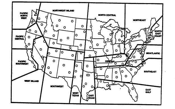
Annual precipitation Where site specific values for P are not available these can be estimated from Figure 1 and Table 1. In Illinois, reasonable estimates fall between 30 inches per year in the northern and central parts of the State to 42 inches per year in the extreme southern section.
FIGURE 1 Rain Zones for the United States (EPA, 1989
TABLE 1 Typical Values for Annual Precipitation
in Rain Zones of the United States (EPA, 1989)
Rain
ZoneNumber of Storms
COV
Precip (in)
COV
Northeast
70
0.13
34.6
0.18
Northeast-
Coastal62
0.12
41.4
0.21
Mid-Atlantic
62
0.13
39.5
0.18
Central
68
0.14
41.9
0.19
North Central
55
0.16
29.8
0.22
Southeast
65
0.15
49.0
0.20
East Gulf
68
0.17
53.7
0.23
East Texas
41
0.22
31.2
0.29
West Texas
30
0.27
17.3
0.33
Southwest
20
0.30
7.4
0.37
West Inland
14
0.38
4.9
0.43
Pacific South
19
0.36
10.2
0.42
Northwest Inland
31
0.23
11.5
0.29
Pacific Central
32
0.26
18.4
0.33
Pacific Northwest
71
0.15
35.7
0.19
COV = Coefficient of Variation = Standard Deviation/Mean
Correction Factor This factor is used to account for smaller storms which produce no runoff. The value of Pj may be estimated to be 0.9 where more precise data are unavailable.
Runoff Coefficient Rv represents that fraction of precipitation which appears as runoff. This may be estimated from the following:
(EQ 2)Rv = 0.05 + 0.009(I) (Schueler, 1987)
where I is the impervious area for the site expressed as percent. I may be estimated by summing the area of impervious surfaces dividing by the total area.
Alternatively, I may be estimated for residential areas by:
(EQ 3) I = 9(PD)1/2 (Shelly, 1988)
where PD is the population density in persons/acre.
Pollutant Concentration The concentration of pollutant C, may be determined from flow-weighted composite samples representative of annual average values in urban runoff from a given area. Where such data are not available, estimates may be based on data from the NURP database or other reliable sources. A table of C values compiled from NURP data is provided in Table 2. Other data on pollutant concentrations (Schueler, 1987), are presented in Tables 3 and 4.
TABLE 2 Water Quality Characteristics of
Urban Runoff from NURP (U.S. EPA, 1983)
Pollutant
For Media
Urban SiteFor 90th
Percentile Urban SiteCoefficient
of VariationTSS (mg/l)
100
300
1-2
BOD (mg/l)
9
15
0.5-1.0
COD (mg/l)
65
140
0.5-1.0
Tot. P (mg/l)
0.33
0.70
0.5-1.0
Sol. P (mg/l)
0.12
0.21
0.5-1.0
TKN (mg/l)
1.5
3.3
0.5-1.0
NO2 + 3 -N (mg/l)
0.68
1.75
0.5-1.0
Copper (ug/l)
34
93
0.5-1.0
Lead (ug/l)
144
350
0.5-1.0
Zinc (ug/l)
160
500
0.5-1.0
TABLE 3 Concentration (C) Values for Use with Simple Method
Pollutant
Residential
Mixed
Commercial
Open/
NonurbanMed
COV
Med
COV
Med
COV
Med
COV
BOD mg/l
10.0
0.41
7.8
0.52
9.3
0.31
--
--
COD mg/l
73
0.55
65
0.58
57
0.39
40
0.78
TSS mg/l
101
0.96
67
1.14
69
0.85
70
2.92
Total P
383
0.69
263
0.75
201
0.67
121
1.66
Soluble P
143
0.46
56
0.75
80
0.71
26
2.11
TKN
1900
0.73
1288
0.50
1179
0.43
965
1.00
Nit.NO2+NO3
736
0.83
558
0.67
572
0.48
543
0.91
Copper ug/l
144
0.75
114
1.35
104
0.68
30
1.52
Lead ug/l
33
0.99
27
1.32
29
0.81
--
--
Zinc ug/l
135
0.84
154
0.78
226
1.07
195
0.66
Source: NURP (EPA 1983)
TABLE 4 Concentration Values for Hardwood Forest (OWML, 1983)
Pollutant
Concentration
COD (mg/l)
>40
Tot. P (mg/l)
0.15
Sol. P (mg/l)
0.04
TKN (mg/l)
0.61
NO2 -N (mg/l)
0.17
EXAMPLE 1
A proposed 25 acre development in Northeastern Illinois would convert a woodland area (I = 2%) to single family homes and townhouses. The total imperviousness would be 40%. Estimate the post-development increases in phosphorus and total Kjeldahl nitrogen (TKN) loadings.
Discussion
The annual precipitation is assumed to be 30 inches/year (Table 1). The runoff coefficient is calculated from EQ 2.
Prior to development, I = 2%:
Rv = 0.05 + 0.009(2) = 0.068
After development:
Rv = 0.05 + 0.009(40) = 0.41
The concentration values C, are taken from Tables 3 and 4. (Mean NURP concentration values are assumed)
Parameter Pre-development Post-development P 30 inches/year 30 inches/year Pj 0.9 0.9 Rv 0.068 0.41 C (TKN) 0.61 mg/l 1.5 mg/l C (total P) 0.15 mg/l 0.33 mg/l A 25 acres 25 acres Annual loadings are computed from EQ. 1:
Pre-development:
TKN = [(30 in/yr)(0.9)(0.068)(0.61 mg/l)(25 acres)(0.227)] = 6.4 lbs/yr
P-total = [(30 in/yr)(0.9)(0.068)(0.15 mg/l)((25 acres)(0.227)] = 1.6 lbs/yr
Post-development:
TKN = [(30 in/yr)(0.9)(0.41)(1.5 mg/l)(25 acres)(0.227)] = 94.2 lbs/yr
P-total = [(30 in/yr)(0.9)(0.41)(0.33 mg/l)((25 acres)(0.227)] = 20.7 lbs/yr
Results:
Parameter Pre-devel. Post-devel. %Increase TKN 6.4 lbs/yr 94.2 lbs/yr 1472% P-total 1.6 lbs/yr 20.7 lbs/yr 1294%
For the above example, what would be the post development nutrient increase if the total imperviousness were limited to 25%?
Discussion
From Equation 2, Rv = 0.28. From Equation 1, the post development increase would be:
Parameter Pre-devel. Post-devel. % Increase TKN 6.4 lbs/yr 64.3 lbs/yr 1000 P-total 1.6 lbs/yr 14.1 lbs/yr 884
EXAMPLE 3
Suggest a BMP or group of BMPs which could potentially limit the export of total phosphorus to within 50 % of pre-development levels.
Discussion
Table 15 provides a summary of pollutant removal efficiencies for various storm water runoff control practices. Wet ponds or multiple pond systems are the most reliable practices for controlling nutrients in runoff, and are also generally effective in removing other pollutants of concern.
Loading Functions The simple method may be used to convert typical concentration values to estimates of annual mass loadings. Also known as loading functions, these estimates can be based upon unit area for various land use types and per cent site imperviousness, or other similar constants. Loading functions allow for a direct estimation of pollutant loading for various land use types. Table 4 presents calculated loading functions from various land use types.
TABLE 4 Calculated Pollutant Mass Loadings for Various Land Uses
(Pounds/Acre/Year)
Land Use
I
Total
Phos.TKN
BOD
5-dayZinc
Lead
Rural
Residential0
5
10
0.10
0.19
0.28
0.45
0.86
1.27
2.70
5.16
7.62
0.05
0.09
0.14
0.04
0.08
0.12
Large Lot Single Family
10
15
20
0.28
0.38
0.46
1.27
1.73
2.09
7.62
10.4
12.5
0.04
0.18
0.22
0.12
0.17
0.20
Medium Density
Single Family
20
25
30
35
0.46
0.55
0.64
0.74
2.09
2.50
2.92
3.36
12.5
15.0
17.5
20.2
0.22
0.27
0.31
0.36
0.20
0.24
0.28
0.32
Town-house
35
40
45
50
0.74
0.83
0.92
1.01
3.36
3.77
4.18
4.59
20.2
22.6
25.1
27.5
0.36
0.40
0.45
0.49
0.32
0.36
0.40
0.44
Garden
Apartment50
55
60
1.01
1.10
1.19
4.59
5.00
5.41
27.5
30.0
32.5
0.49
0.53
0.58
0.44
0.48
0.52
High Rise,
Light Commercial/ Industrial60
65
70
75
80
1.19
1.28
1.37
1.46
1.55
5.41
5.82
6.23
6.64
7.05
32.5
34.9
37.4
39.8
42.3
0.58
0.62
0.66
0.70
0.75
0.52
0.56
0.60
0.64
0.68
Heavy Commercial, Shopping Center
80
85
90
95
100
1.55
1.64
1.72
1.82
1.91
7.05
7.45
7.82
8.27
8.68
42.3
44.7
46.9
49.6
52.1
0.75
0.80
0.83
0.88
0.93
0.68
0.72
0.75
0.79
0.83
1
P=30 inches, Pj=0.9, Rv=0.05+0.009(I), A= 1 acre,C= mean NURP values from Table 2
Similar loading functions can be made using the data in Table 3 or other appropriate data.
Total annual loads are estimated by multiplying the area associated with each given land use type by the loading function for that land use:
(EQ. 4) L = SUM (Lx)(Ax)
where:
L = total loading (lbs/yr)
Lx = loading function for land use x (lbs/acre/yr)
Ax = area of land use x (acre)
In another variation of the Simple Method, Heaney (Mills et al, 1985) has developed a loading function based on population density and street cleaning frequency:
Lx = (ax)(Fx)(Yx)(P)(EQ.5)
where:
Lx = loading function for land use x (lbs/acre)
ax = pollutant concentration factor (lbs/acre/in)
Fx = population density function
Yx = street cleaning factor
P = annual precipitation (inches)
Total loading is calculated using EQ. 5. Typical ax values are given in Table 5.
TABLE 5 Pollutant Concentration Factors (ax)
For use in EQ 5
Land Use
BOD
TSS
PO4
Nit.
Residential
0.78
16
0.033
0.13
Commercial
3.13
22
0.073
0.29
Industrial
1.18
29
0.069
0.27
Other Developed
0.11
2.7
0.009
0.06
The population density function, Fx is a dimensionless parameter. Typical empirical values for Fx adapted from Heaney et al. are:
for commercial and industrial development, and1.0
(EQ. 6) 0.142 + 0.134 [0.405(PD)]0.54 for residential
where:
PD = population density (persons/acre)
The street cleaning factor is based upon the street sweeping interval in days (Ns):
= Ns/20 for Ns < 20 daysYx
Yx = 1.0 for Ns > 20 days
EXAMPLE 4
Referring to Example 1, assume that the population density is 25 persons/acre and that street sweeping is performed 1/month, what is the annual nitrogen and phosphorus loading from the development as predicted from EQ. 4 ? How does this compare with the prediction from Example 1?
ANSWER
From TABLE 4, ax is 0.033 (lbs/acre/in).
From EQ. 6, the population density function, Fx = 0.87
Yx is set to 1.0, since street sweeping frequency is less than 1/20 days.
P = 30 in/yr.
From EQ 5, the phosphorus loading function is:Lx = (0.033 lbs/acre-inch)(0.87)(1.0)(30 in/yr) = 0.86 lbs/acre-yr
The total annual load from EQ 3 is:
L = (25 acres)(0.86 lbs/acre-yr) = 22 lbs/yr (Using the simple method in Example 1 predicted 20.7 lbs/yr)
2. PHOSPHORUS LOAD ALLOCATIONS - THE MAINE DEP METHOD
The Maine Department of Environmental Protection has developed a detailed application of the loading functions method for determining changes in phosphorus loadings which may be expected as a result of different urban and suburban development scenarios (Dennis et al. 1989). Estimated phosphorus loadings can be compared with specified phosphorus loading allocations for Maine lakes. In addition, the procedure allows for the estimation of phosphorus loading mitigation, based on the use of various combinations of BMPS. By use of simple desk-top calculations, planners and developers are able to estimate in advance whether proposed development areas will comply with the State's phosphorus loading allocations.
The acceptable increase in phosphorus export is determined by:
Lp = (FC)/D(EQ. 7)
where:
Lp = acceptable increase in the phosphorus loading function (lbs/acre/yr)
1
F = phosphorus coefficient for the lake watershed (lbs/ppb/yr)C = acceptable increase in lake phosphorus concentration (ppb)
D = future area to be developed over next 50 years in the watershed (acres)
1
F factors have been determined for specific lakes in Maine. Similar targets may be established for waterbodies in other areas. In the absence of specific loading limitations, the process may be used to estimate the increase in phosphorus loading resulting from a proposed development.C, the acceptable increase in phosphorus concentration, is a function of existing water quality and the level of desired protection. C values are given in Table 6.
TABLE 6 C Values - Acceptable Increase in Lake Phosphorus Concentration
(Maine DEP, 1989)
Water Quality Category
Lake Protection Level
High
Medium
Low
Outstanding
0.5
1.0
1.0
Good
1.0
1.5
2.0
Moderate/Stable
1.0
1.25
1.5
Moderate/Sensitive
0.75
1.0
1.25
Poor/Restorable
0.1
0.5
NA
Poor/Low Priority
2.0
4.0
6.0
D
is determined as the total area minus already developed and undevelopable land (steep slopes, wetlands, parks, etc.) and multiplying by a development factor which estimates the portion of undeveloped land which is likely to be developed. In Maine these development factors are:for lake areas near growth centers0.20 - 0.35
0.15 - 0.25 for lake areas subject to seasonal development
0.10 - 0.20 for lakes for which development is shoreline dependent
0.10 - 0.15 for lake areas not subject to development pressure
It is recommended that conservative upper estimates be used for development factors.
The permitted phosphorus export (PPE) for a site is simply:
(EQ. 8) PPE = (Lp)(A)
where:
PPE = permitted phosphorus export for proposed development (lbs/acre)
A = the proposed area of the site (acres)
The proposed area of the development (A) should include all areas except those which are undevelopable such as wetlands > 1 acre, and steep slopes.
The total predicted phosphorus export (TE) for a development site is the summation of export values from roadways, individual houselots, multi-unit housing, commercial and industrial development. Credit is given for phosphorus control measures which are employed. The general equation for Phosphorus export is:
(EQ. 9) (TE) = summation (RE) + (HE) + (CE)
where:
(TE) = total predicted phosphorus export
(RE) = phosphorus export from roadways
(HE) = phosphorus export from individual house lots
(CE) = phosphorus export from multi-unit housing, commercial, and industrial development,
Phosphorus Export from Residential Area Roadways (RE)
Road surface phosphorus export is determined as follows:
(RE) = [(FT)(LBS)(TFb)(TFwp)(TFi)(TFo)]/100(EQ. 9)
where:
(FT) = length of roadway being evaluated (feet)
(LBS) = annual export of phosphorus from 100 feet of roadway, before treatment
(TFb) = treatment factor for buffer strips
(TFwp) = treatment factor for wet ponds
(TFi) = treatment factor for infiltration practice
(TFo) = treatment factor for other treatment factor
The annual export per 100 feet of roadway is calculated as:
(LBS) = (road surface width)(0.012) + (road ditch width)(0.004)(EQ. 10)
Treatment factors (TF) for all the above calculations and those that follow must be numbers between 0 and 1.0 which reflect the long term phosphorus removal efficiency of the treatment practice or practices employed. Tables in Appendix C-1 present some recommended values. Note that lower numbers reflect higher removal efficiencies. It is also evident that the calculation gives greater credit where redundant treatment practices are employed.
Phosphorus export from individual house lots (HE)
The annual phosphorus export from an individual houselot is calculated as:
(EQ. 11) (HE) = (BP)(TFb)(TFwp)(TFi)(TFo)
where:
(BP) = phosphorus export before treatment
(TFb) = treatment factor for buffer strips
(TFwp) = treatment factor for wet ponds
(TFi) = treatment factor for infiltration practice
(TFo) = treatment factor for other treatment factor
Table 11 presents (BP) values for different hydrologic groups
TABLE 11 Phosphorus Export (BP Values) From Lots
Before Treatment - Residential
Hydrologic Group
Area Cleared per Lot
<10,000 ft
>10,000 ft
>15,000 ft
A
.27 (.2)
.30 (.30)
.35 (.35)
B
.32 (.40)
.39 (.46)
.49 (.54)
C
.34 (.48)
.44 (.56)
.58 (.67)
D
.36 (.62)
.47 (.62)
.62 (.74)
Note:
Values in parentheses are appropriate for sites where more than 40% of timber volume has been harvested within the last 5 years.Phosphorus Export from Multi-unit Housing, Commercial, and Industrial Development (CE)
Phosphorus Export from multi-unit housing, commercial, and industrial development is calculated as:
(EQ. 12) (CEx) = (Lx)((BLx)(TFb)(TFwp)(TFi)(TFo)
where:
(Lx) = altered land surface area (acres)
(BLx) = additional phosphorus export per acre of altered land surface (lbs/acre)
(TFb) = treatment factor for buffer strips
(TFwp) = treatment factor for wet ponds
(TFi) = treatment factor for infiltration practice
(TFo) = treatment factor for other treatment factor
Values for additional phosphorus export associated with altered land uses are found in Table 12.
TABLE 12 Phosphorus Export from Altered Land Uses
Land Use Category
Phosphorus Export Before Treatment
Lawn A
.30 lbs/acre
Lawn B
.65 lbs/acre
Lawn C
.97 lbs/acre
Lawn D
1.1 lbs/acre
Road Ditch
1.8 lbs/acre
Road Surface
5.3 lbs/acre
Impervious Surfaces
3.5 lbs/acre
The total loading from multi-unit housing, commercial and industrial areas is the summation of all areas for various land use categories.
EXAMPLE 5
Referring to the proposed development in Example 1, consists of 40 single family units with an average lot size of 0.31 acres, and 29 townhouses with an average of 0.43 acres. The resident soil is Type C. All the runoff will be treated by a wet detention basin. Runoff from the townhouses and roads will also be treated by a 150 foot buffer strip with a slope of 12%. The wet detention basin will be designed with a length to width ratio of 3:1, and mean depth of 5 ft.
The total road length to be added as part of the subdivision is 1,100 feet. The road width is 38 feet with 4 foot shoulders. The main access road which is included in the total road length is 700 feet and has 5 foot ditches on each roadside.
Calculate the additional phosphorus export associated with the proposed development. Also calculate without treatment and compare with Examples 1 and 4.
Discussion
Referring to Appendix C-1, assume a treatment factor of 0.7 for buffer strips 0.5 for the wet detention pond. The analysis must consider the runoff from the houses and townhouses separately. Assuming that < 10,000 ft2 cleared, phosphorus loading from the single-family dwellings is:
(HE) = (40 lots)(0.48lbs/lot/yr)(0.5) = 9.6 lbs/yr
From the townhouses:
(CE) = (29 lots)(0.43 acres/lot)(0.97 lbs/acre/yr)(0.5)(0.7) = 4.2 lbs/yr
For the roadways, use EQ. 9:
(LBS) = [(38 + 4 + 4)(0.012)] + [(5 + 5)(0.004)] = 0.59 lbs/100 ft
(RE) = (11)(0.59)(0.7)(0.5) = 2.3 lbs/yr
The total additional phosphorus export is then:
HE + CE + RE = 16.1 lbs/yr
Without treatment:
(HE) = (40 lots)(0.48lbs/lot/yr) = 19.2 lbs/yr
From the townhouses:
(CE) = (29 lots)(0.43 acres/lot)(0.97 lbs/acre/yr) = 12.1 lbs/yr
For the roadways, use EQ. 9:
(LBS) = [(38 + 4 + 4)(0.012)] + [(5 + 5)(0.004)] = 0.59 lbs/100 ft
(RE) = (11)(0.59) = 6.5 lbs/yr
The total additional phosphorus export is then:
HE + CE + RE = 37.8 lbs/yr
This is somewhat higher than the solutions to Examples 1 and 4 (20.7 lbs/year and 22 lbs/year, respectively).
EXAMPLE 6
A 7.4 acre office complex in an area with type B soils is proposed. The site includes 4.9 acres of lawn area. Rooftop accounts for 0.9 acres. and 1.1 acre for parking, and 0.3 acres for road surface, and 0.2 acres for road ditch. Calculate the additional phosphorus export.
All flows are to be treated by a 100 ft buffer strip with 10% slope and a wet detention pond with a 4:1 length to width ratio and a mean depth of 4 feet.
Discussion
From Appendix C - 1, TABLES C - 1.1 and C - 1.2, the Treatment factors are 0.6 for the buffer strip and 0.48 for the wet pond. Phosphorus loadings from the various areas are from Table 12 and EQ 9. The total loading is:
(CE) = [(4.9)(0.65) + (0.9)(3.5) + (1.1)((3.5) + (0.3)(5.3) + (0.2)(3.5)] x [(0.6)(0.48)] = 2.77 lbs phosphorus/yr
Other pollutants
While the Maine procedure was conceived for use in loading estimates of a particular pollutant (phosphorus), and is specific to the State of Maine, the basic concept can be expanded for use with other pollutants of concern in any type of receiving water anywhere in the country. In order to adapt this procedure, the following types of information are necessary:
- Data on annual average loading per unit area for given types of land uses.
- Data on the treatment efficiency of various best management practices in reducing the loading of pollutants of concern.
Where available, these may be compared with target loading ceilings for pollutants of concern.
Table 13 summarizes data on concentrations of various pollutants in runoff from to urban catchments in Wisconsin (Bannerman et al, 1992). In Table 14 these are converted to annual pollutant load per acre, based on 30 inches of precipitation annually. These can be converted to lbs per square foot by dividing by 43,560.
TABLE 13 Pollutant Concentrations from Various Source
Areas in Two Urban Catchments in Wisconsin
Source1
Mean Pollutant Concentration2
TSS
mg/lTotal
Phos mg/lCd
ug/lCr
ug/lCu
ug/lPb
ug/lZn
ug/lIndustRoof 1
54
.13
.3
--
7
8
1348
Arterial ST 1
875
1.01
2.8
26
85
85
629
Arterial ST 2
241
.53
2.6
18
50
55
554
Feeder ST 1
969
1.57
3.7
17
97
107
574
Feeder ST 2
1085
1.77
.8
7
25
38
245
Parking Lot 1
475
.48
1.2
16
47
62
361
Parking Lot 2
91
.26
.08
7
21
30
249
Outfall 1
174
.38
1.1
7
31
26
295
Outfall 2
374
.86
.6
5
20
40
254
ResiDriveway 2
193
1.5
.5
2
20
20
113
FlatRoof 2
19
.24
.4
--
10
10
363
Collector ST 2
386
1.22
1.7
13
61
62
357
ResiLawn 2
457
3.47
--
--
13
--
60
ResiRoof 2
36
.19
.2
--
5
10
153
Source: Bannerman et al, 1992
1
Study area 1 described as mainly industrial; Study area 2 described as medium density residential2
Area = 1 acre P = 30 inches/yr
TABLE 14 Pollutant Loadings per Acre From Various Sources,
Based on Wisconsin Data
Source1
Pollutant Loading (lbs/acre/year)2
TSS
Total
Phos
Cd
Cr
Cu
Pb
Zn
IndustRoof 1
367
.88
.002
--
.05
.05
9.2
Arterial ST 1
5950
6.9
0.2
.18
.58
.58
4.3
Arterial ST 2
1639
3.6
.018
.12
.34
.37
3.8
Feeder ST 1
6589
10.7
.025
.12
.66
.73
3.9
Feeder ST 2
7378
12.0
.005
.05
.17
.26
1.67
Parking Lot 1
3230
3.26
.008
.11
.32
.42
2.45
Parking Lot 2
619
1.77
.0005
.05
.14
.20
1.69
Outfall 1
1183
2.58
.007
.05
.21
.18
2.01
Outfall 2
2543
5.84
.004
.03
.136
.27
1.73
ResiDriveway 2
1312
10.2
.003
.014
.136
.136
.768
FlatRoof 2
129
1.63
.003
--
.068
.068
2.47
Collector ST 2
2625
8.30
.012
.088
.415
.422
2.43
ResiLawn 2
3108
23.6
--
--
.088
--
0
ResiRoof 2
245
1.29
.0014
--
.034
.068
1.04
Source: Bannerman et al, 1992
1
Study area 1 described as mainly industrial; Study area 2 described as medium density residential2
Area = 1 acre P = 30 inches/yearSchueler has provided an assessment of effectiveness of various control practices in removing pollutants (Schueler, 1992). A summary is provided in Table 15.
TABLE 15 Pollutant Removal Efficiencies For Various Control Practices
Storm Water Management
PracticePollutant Removal Efficiency
TSS
Nutrients
Organic
Metals
Extended Detention
30-70%
low to neg.
for soluble
nutrients
15-40%
for COD
Wet Ponds
50-90%
30-90% for
total P
40-80% for
sol. nutr.
mod-high
removal
mod-high
removal
Stormwater Wetlands
slightly
higher than
wet ponds
somewhat
lower than
wet ponds
Multiple Pond System
Varies with design, but typically enhanced
over individual pondsInfiltration Trenches
+90%
60%
+90%
Infiltration Basins
Porous Pavement
up to 80%
up to 60%
for Phosup to 80%
for NitHigh
High
Sand Filters
85%
40% for dissolved
Phosphorus35% for Nit
50-70%
Peat Sand Filters
85%
70% for Phosphorus
50% for Nit
90% for
BOD
Grassed Swales
up to 70%
30% for Phos
25% for Nit
50-90%
Filter Strip
28%
Source: Schueler et al, 1992
EXAMPLE 7
Returning to Example 1 and Example 5. Assume that the single family units have roofs which are 2,400 square feet (0.055 acre), and the townhouse roofs are 3,000 square feet (0.069 acre). Residential driveways are assumed to average 610 square feet (0.014 acres). Parking for the townhouses consists of 11 lots at an average of 6,500 square feet (0.15 acres) each.
Calculate the zinc loading for the 25 acre single family/townhouse development, using the Tables 14 and 15, and alternatively, EQ 1, before treatment. How do the results compare?
Discussion
The total roof area is:
(40)(0.055) + (29)(0.069) = 4.2 acres rooftops
Total driveway area is:
(40)(0.014 acres) = 0.56 acres driveway
Total parking lot area is:
(11)(0.15 acres) = 1.65 acres parking lot.
The area associated with the roadways (feeder street) is:
(38 + 4 + 4)(1,100) = 50,600 square feet or 1.2 acres
The remaining area is considered to be residential lawn:
25 - [4.2 + 0.56 + 1.65 + 1.2] = 17.4 acres residential lawn
Loading estimates:
Referring to Table 14, the estimated loading rate from rooftops is assumed to be 1.04 lbs zinc/yr, and 0.68 lbs lead/yr. Total loading for the development is:
Zinc - (4.2 acres)(1.04 lbs/acre/yr) = 4.24 lbs/yr
Lead - (4.2 acres)(0.68 lbs/acre/yr) = 2.86 lbs/yr
The estimated loading rate from residential driveways is assumed to be 0.768 lbs zinc/acre/yr, and 0.136 lbs lead/acre/yr. Total loading from residential driveways is:
Zinc - (0.56 acres)(0.768 lbs/acre/yr = 0.43 lbs/yr
Lead - (0.56 acres)(0.136 lbs/acre/yr = 0.076 lbs/yr
The estimated loading rate from parking lots is 1.69 lbs zinc/acre/yr and 0.20 lbs lead/acre/yr (assume study area 2 - medium density residential). Total loading from parking lots is:
Zinc - (1.65 acres)(1.69 lbs/acre/yr) = 2.60 lbs/yr
Lead - (1.65 acres)(0.20 lbs/acre/yr) = 0.33 lbs/yr
The estimated loading rate from the feeder streets is 1.67 lbs zinc/acre/yr, and 0.26 lbs lead/acre/yr. Total loading is:
Zinc - (1.2 acres)(1.67 lbs/acre/yr) = 2.00 lbs/yr
Lead - (1.2 acres)(0.26 lbs/acre/yr) = 0.31 lbs/yr
The estimated loading rate from residential lawns is 0 for zinc and unknown for lead. Therefore, assume no significant increase in metals loading from these areas.
Summing the above the total loading from all areas is gives:
- 4.24 + 0.43 + 2.60 + 2.00 = 9.3 lbs/yrZinc
Lead - 2.86 + 0.076 + 0.33 + 0.31 = 3.6 lbs/yr
Using EQ 1a, and referring back to Table 2 and Example 1:
= (30 in/yr)(0.9)(0.068)(0.160 mg/l)(25 acres) = 7.3 lbs/yrZinc
Lead = (30 in/yr)(0.9)(0.068)(0.144 mg/l)(25 acres) = 6.6 lbs/yr
The methods provide reasonable agreement for the proposed development.
3. ESTIMATING ACUTE CONCENTRATIONS
The approaches outlined above offer tools for predicting changes in long-term loading rates of pollutants to surface waters as an aid to planning activities. These methods do not provide for estimating short term impacts of urban runoff. Such impacts are more properly viewed as the result of instream pollutant concentrations rather than average loading rates. Predicted instream concentrations can be compared with state water quality standards as a means of predicting water quality standards violations due to urban runoff.
Typically much more complex computer models are employed to predict short term wet weather impacts to receiving waters brought about by urbanization. These models integrate hydrological and instream chemical processes in order to estimate instream pollutant concentrations. Models such as STORM and SWMM require significant data input and site specific verification.
Analysis of data collected as part of the National Urban Runoff Program (NURP) indicates that event mean pollutant concentrations may adequately be specified as a lognormal distribution (EPA, 1986). Because of this, the expected concentration for a given probability for a given pollutant in urban runoff can be determined for a particular data set if the central tendency (median or mean value) and the variability (coefficient of variation or standard deviation) are known. This concentration can be compared to some reference concentration such as a water quality standard to indicate the likelihood that an acute water quality impact will occur in the receiving water. Alternatively, the probability that a given concentration level (such as a water quality standard) will be exceeded can be estimated.
The expected runoff concentration for pollutant x is:
(EQ. 13) Cx = Cm (exp [Z (ln{1+COV}2)1/2]
where:
* Cx = expected concentration of pollutant x
* Z = standard normal probability (for specified probability of occurrence)
* Cm = median pollutant concentration
* COV = coefficient of variation
* For log-transormed data
The probability that a specified concentration will be exceeded can be determined by substituting the concentration level of interest for Cx in EQ. 13, solving the equation for Z, and locating the associated probability for the calculated Z value:
(EQ. 14) Z = (ln[Cx/Cm])/[(ln(1+COV2)1/2]
Z values for various probabilities of occurrence is presented in Table 16.
Median event mean concentrations and coefficients of variation for NURP data for all land use types are presented in Table 3. If sufficient local data are available these may also be used provided they are transformed into logrhythmic form. Illinois Water quality standards for various pollutants is presented in Table 17. For certain metals these are based on hardness.
TABLE 16 Z Values for Various Probabilities
Z Value
Probability of Exceedance
3.090
0.1%
2.326
1%
2.054
2%
1.881
3%
1.751
4%
1.645
5%
1.476
7%
1.282
10%
1.036
15%
0.842
20%
0.674
25%
0.524
30%
0.385
35%
0.253
40%
0.000
50%
-0.253
60%
-0.524
70%
-0.842
80%
-1.282
90%
TABLE 17 Illinois Water Quality Standards
Pollutant
Acute Standard
Chronic Standard
Arsenic (ug/l)
360
Cadmium (ug/l)
exp[A + B ln(H)]
but not > 50ug/l
A=-2.98, B=1.128
exp[A + B ln(H)]
A=-3.49, B=0.785
Hexavalent Chromium (ug/l)
16
11
Trivalent Chromium (ug/l)
exp[A + B ln(H)]
A=3.688, B=0.819
exp[A + B ln(H)]
A=1.561, B=0.819
Copper (ug/l)
exp[A + B ln(H)]
A=-1.46, B=0.942
exp[A + B ln(H)]
A=-1.47, B=0.855
Cyanide (ug/l)
22
5.2
Lead (ug/l)
exp[A + B ln(H)]
but not >100ug/l
A=-1.46, B=1.273
NA
Mercury (ug/l)
0.5
NA
Barium (mg/l)
5.0
NA
Boron (mg/l)
1.0
NA
Chloride (mg/l)
500
NA
Fluoride (mg/l)
1.4
NA
Iron Mg/l)
1.0
NA
Manganese (mg/l)
1.0
NA
Nickel (mg/l)
1.0
NA
Phenols (mg/l)
0.1
NA
Selenium (mg/l)
1.0
NA
Silver (ug/l)
5.0
NA
Sulfate (mg/l)
500
NA
Total Dissolved Solids (mg/l)
1000
NA
Zinc (mg/l)
1.0
NA
H = Hardness
EXAMPLE 8
For the development described in Example 1, what is the probability that water quality standards will be violated for zinc and lead, assuming no treatment.
Answer
From Table 15, the acute water quality standard for lead is:
WQSacute = exp[-1.46 + 1.273(ln(H))]
Assuming the Hardness = 100 mg/l, then:
WQSacute = 82 ug/l lead
From Table 15, the acute water quality standard for zinc is:
WQSacute = 1.0 mg/l zinc
From Table 3, the median concentrations and Coefficients of variation for lead and zinc are
Lead: Cm = 33 ug/l, COV = 0.99
Zinc: Cm = 135 ug/l, COV = 0.84
Applying EQ 14, the probability that lead and zinc water quality standards would be exceeded for any given storm (assuming no treatment or dilution) would be estimated to be:
Lead: Z = (ln[82/33])/[(ln(1+ 0.99)2)]1/2
Z = 0.77, which corresponds to an exceedance probability of 20 - 25%
Zinc: Z = (ln[1000/135])/[(ln(1+ 0.84)2)]1/2
Z = 1.81, which corresponds to an exceedance probability of less than 5%
REFERENCES
Bannerman, R.T., Dodds, R., Owens, D., Hughes, P. 1992. Sources of Pollutants in Wisconsin Stormwater. Wisconsin Department of Natural Resources Grant Report.
Dennis, J., Noel, J., Miller, D., Eliot, C. 1989. Phosphorus Control in Lake Watersheds: A Technical Guide to Evaluating New Development. Maine Department of Environmental Protection.
Mills, W.B., Porcella, D.B., Ungs, M.J., Gherini, S.A., Summers, K.V., Mok, L, Rupp, G.L., Bowie, G.L., Haith, D.A. Water Quality Assessment: A Screening Procedure for Toxic Pollutants. EPA - 600/6-85-002A
Scheuler, T.R. 1987. Controlling Urban Runoff: A Practical Manual for Planning and Designing Urban BMPs. Metropolitan Washington Council of Governments.
Scheuler, T.R., Kumble, P.A., Heraty, M.A. 1992. A Current Assessment of Urban Best Management Practices. Techniques for Reducing Non-Point Source Pollution in the Coastal Zones. Metropoltan Washington Council of Governments.
Shelly, P. Technical Memorandum to S.A.I.C, 11/03/88.
U.S. Environmental Protection Agency (EPA). 1983. Results of the Nationwide Urban Runoff Program. Volume I. Final Report. Water Planning Division. Washington, D.C.
U.S. Environmental Protection Agency (EPA). Urban Targeting and BMP Selection. Terrene Institute, Washington, D.C.
APPENDIX C-1 -- TREATMENT FACTORS FOR USE IN MAINE DEP PROCEDURE
TABLE C-1.1 Treatment Factors (TF) for Buffer Strips
Hydrologic Group A Soils
Treatment Factor- Wooded (Non-Wooded)
Slope
25 ft
50 ft
100 ft
150 ft
200 ft
0-10%
.75 (.95)
.4 (.6)
.2 (.4)
.1 (.3)
0 (.2)
11-15%
.8 (1.0)
5. (.7)
.25 (.45)
.1 (.3)
0 (.2)
16-20%
.8 (1.0)
.7 (.9)
.5 (.7)
.25 (.45)
.1 (.3)
21-30%
.8 (1.0)
.75 (.95)
.7 (.9)
.6 (.8)
.3 (.6)
Hydrologic Group B Soils
Treatment Factor- Wooded (Non-Wooded)
Slope
25 ft
50 ft
100 ft
150 ft
200 ft
0-10%
.75 (.95)
.6 (.8)
.4 (.6)
.2 (.4)
.1 (.2)
11-15%
.8 (1.0)
.75 (.95)
.5 (.7)
.2 (.4)
.1 (.2)
16-20%
.8 (1.0)
.8 (.1.0)
.65 (.85)
.4 (.6)
.2 (.4)
21-30%
.8 (1.0)
.8 (.1.0)
.7 (.9)
.5 (.7)
.3 (.6)
Hydrologic Group C Soils
Treatment Factor- Wooded (Non-Wooded)
Slope
25 ft
50 ft
100 ft
150 ft
200 ft
0-10%
.8 (1.0)
.7 (.9)
.55 (.75)
.45 (.65)
.35 (.55)
11-15%
.8 (1.0)
.75 (.95)
.6 (.8)
.5 (.7)
.4 (.65)
16-20%
.8 (1.0)
.8 (1.0)
.7 (.9)
.6 (.8)
.5 (.65)
21-30%
.8 (1.0)
.8 (1.0)
.75 (.95)
.65 (.85)
.5 (.75)
Hydrologic Group D Soils
Treatment Factor- Wooded (Non-Wooded)
Slope
25 ft
50 ft
100 ft
150 ft
200 ft
0-10%
.9 (1.0)
.8 (.65)
.75 (.8)
.7 (.8)
.6 (.75)
11-15%
.9 (1.0)
.85 (1.0)
.8 (.9)
.75 (.9)
.65 (.8)
16-20%
.9 (1.0)
.9 (1.0)
.85 (1.0)
.8 (1.0)
.7 (.85)
21-30%
.9 (1.0)
.9 (1.0)
.9 (1.0)
.8 (1.0)
.75 (.9)
Source: Maine DEP, 1989
TABLE C-1.2 Treatment Factors (TF) for Wet Ponds Volume Treated in One Wet Pond
>4:1 length:width (100% plug flow)
Number of Storm Volumes
1/2 V
1V
2V
3V
MEAN
DEPTH3 ft
.50
.4
.33
.31
5 ft
.47
.34
.27
.24
7 ft
.44
.32
.24
.20
4:1-2:1 length:width (50% plug flow)
Number of Storm Volumes
1/2 V
1V
2V
3V
MEAN
DEPTH3 ft
.56
.48
.42
.40
5 ft
.52
.43
.36
.33
7 ft
.51
.41
.33
.29
<2:1 length:width (100% mixed)
Number of Storm Volumes
1/2 V
1V
2V
3V
MEAN
DEPTH3 ft
.61
.55
.51
.49
5 ft
.59
.51
.45
.43
7 ft
.58
.49
.42
.39
Volume Distributed Between Two Wet Ponds
>4:1 length:width (100% plug flow)
Number of Storm Volumes
1/2 V
1V
2V
3V
MEAN
DEPTH3 ft
.46
.34
.26
.23
5 ft
.43
.31
.22
.18
7 ft
.43
.30
.19
.16
4:1-2:1 length:width (50% plug flow)
Number of Storm Volumes
1/2 V
1V
2V
3V
MEAN
DEPTH3 ft
.50
.39
.31
.28
5 ft
.48
.35
.26
.23
7 ft
.47
.34
.24
.22
<2:1 length:width (100% mixed)
Number of Storm Volumes
1/2 V
1V
2V
3V
MEAN
DEPTH3 ft
.53
.43
.36
.34
5 ft
.52
.41
.33
.30
7 ft
.51
.40
.31
.26
Volume Distributed Between Three Wet Ponds
>4:1 length:width (100% plug flow)
Number of Storm Volumes
1/2 V
1V
2V
3V
MEAN
DEPTH3 ft
.44
.33
.23
.19
5 ft
.43
.30
.19
.16
7 ft
.42
.27
.18
.15
4:1-2:1 length:width (50% plug flow)
Number of Storm Volumes
1/2 V
1V
2V
3V
MEAN
DEPTH3 ft
.47
.35
.26
.23
5 ft
.46
.33
.23
.19
7 ft
.46
.32
.22
.18
<2:1 length:width (100% mixed)
Number of Storm Volumes
1/2 V
1V
2V
3V
MEAN
DEPTH3 ft
.50
.39
.31
.27
5 ft
.49
.36
.27
.24
7 ft
.48
.35
.26
.22